3PL Models Compared for Reverse Logistics Carbon

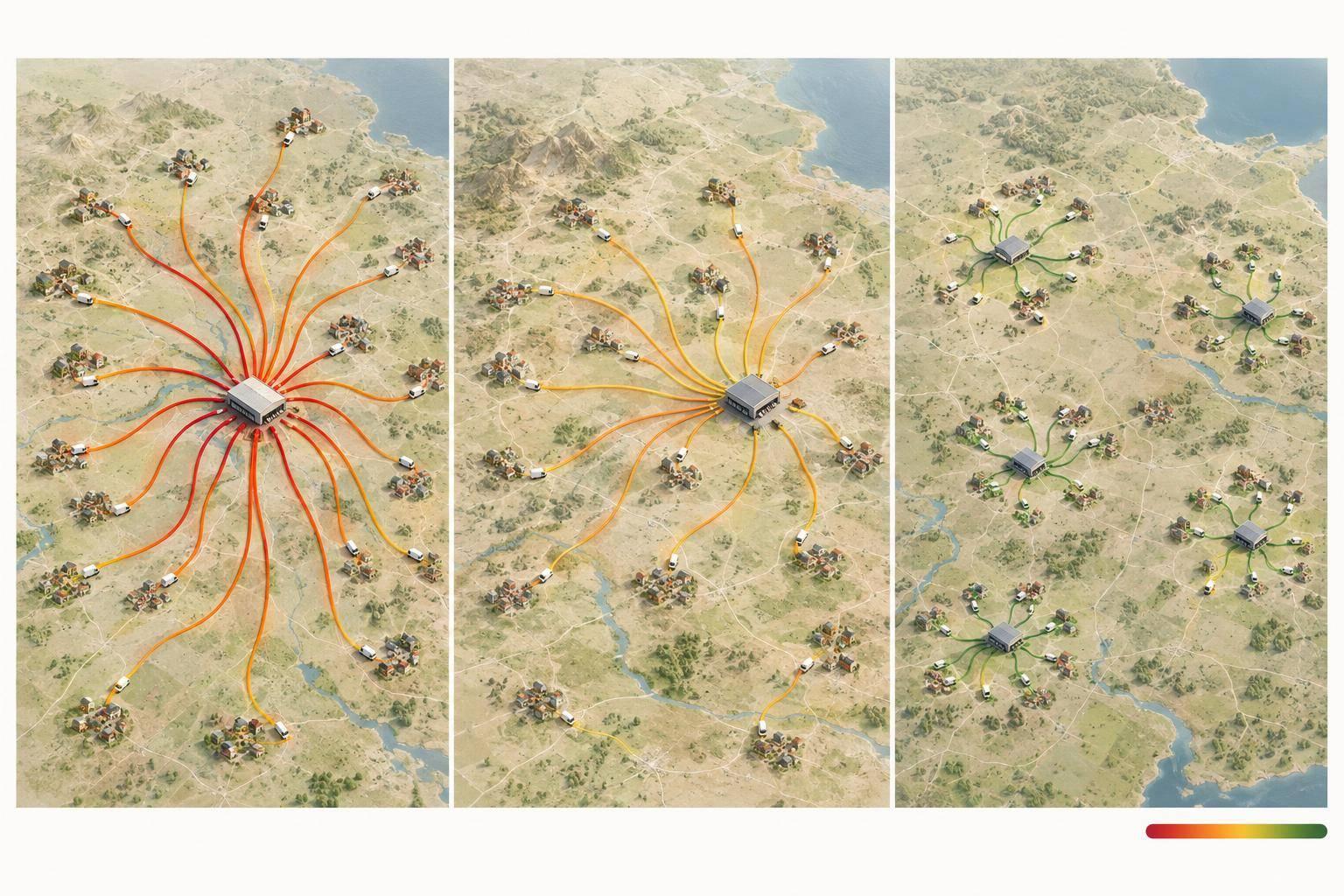
I’d choose a returns model by CO₂e per completed return - not by the number of warehouses. Compare the same products and volumes, count the entire return journey, and track total annual emissions too.

Here’s how I’d weigh the three options:

• In-house returns: More control over inspection and repair, but longer customer shipping trips may offset fewer handoffs.
• Single-node 3PL: Centralized grading and fuller loads may cut emissions - if those savings outweigh longer inbound trips.
• Multi-node 3PL: Nearby sites may shorten shipping distances and support local resale, but transfers add miles and handling.

For each model, I’d check transport miles, load utilization, handling steps, processing time, recovery routes, and data quality. For example, EPA guidance puts pickup and delivery at roughly 30% of an individual LTL shipment’s CO₂ emissions - so distance alone won’t tell you which route wins.

My rule: <u>count emissions through documented final disposition</u>, report any avoided-production credits separately, and test matched return groups before changing your network.

1. In-House Returns

Transport Miles and Consolidation

An in-house returns site can mean fewer handoffs - but longer trips if customers must ship everything to one facility. Low return density can also leave trucks partially loaded or empty on return trips.

Track average miles, shipment weight, load factor, parcel vs. LTL mix, and consolidation rate. EPA SmartWay methodologies use total miles, ton-miles, payload, and carrier activity data to estimate freight emissions. Weigh fewer handoffs against longer shipping distances. Fewer miles only help if processing stays fast.

Processing Time and Handling Steps

Your team's product knowledge can cut repeat inspections and unneeded tests. Map each step from receiving to final shipment, then remove duplicate handling.

Set a 24–48-hour inspection target for priority SKUs and add staff for holiday surges. Faster inspections help keep products eligible for resale and avoid rework. But fixed staffing can slow returns when they compete with outbound orders.

Secondary-Market Routing

After inspection, routing determines whether a return travels extra miles. Use product specifications, warranty rules, and sales data to send eligible items straight to restock or repair. Before choosing liquidation, count downstream transport miles.

A ClearCycle study found 4.3 kg CO₂e per product through a secondary returns processor, compared with about 26 kg through auction liquidation. That result reflects routing choices, not ownership alone.

Data Visibility and Carbon Reporting

You need data to track what routing and handling decisions change. Link each return authorization to shipment, inspection, handling, packaging, and disposition data. Allocate facility energy consistently between returns and outbound work.

Count company vehicles in Scope 1, electricity in Scope 2, and outsourced freight in Scope 3. Outsourcing does not remove emissions.

sbb-itb-eafa320

2. Single-Node 3PL Returns

Compared with in-house returns, the carbon question is straightforward: Does centralized processing offset the extra miles from customers to the facility?

Transport Miles and Consolidation

A single node can increase customer-to-facility miles while improving outbound load density and trailer fill. Compare transport miles, labor touches, processing time, secondary routing, and reporting with the in-house baseline.

EPA guidance says LTL pickup and delivery operations account for roughly 30% of an individual LTL shipment’s CO₂ emissions. Centralized scheduled pickups and backhaul capacity can help cut that share. But fewer truck departures aren't enough. Require lane-level evidence that consolidation offsets the extra customer-to-node miles.

If the mileage benefit holds, check whether the single node also cuts inspection and routing time.

Processing Time and Handling Steps

Dedicated stations and standardized grading can reduce handling, but a single site can become a bottleneck during peak season. Use pre-arrival return data to sort products into unopened, repairable, and end-of-life streams.

Track touches per unit, rework rate, and dwell time to check whether specialized workflows reduce handling and time in storage.

Secondary-Market Routing

Pooling returns can help fill loads bound for refurbishers, resale buyers, or recyclers. Grade products as soon as they arrive and identify the recovery channel that offers the most value.

Compare destination miles and emissions before deciding whether to ship now or wait for consolidation. Wait only when freight savings outweigh emissions from added storage and extra miles, along with any loss of recovery value. Shipment-level visibility lets you test whether consolidation actually lowers carbon emissions.

Data Visibility and Carbon Reporting

Require exportable shipment records that connect each return to its final destination - not just its arrival at the facility. Report inbound freight, processing, outbound recovery shipments, packaging, and disposal separately.

Verifying a single-node 3PL’s carbon results requires third-party records that track the full path from receipt to final disposition.

The next comparison is whether splitting volume across multiple nodes cuts distance enough to offset added transfers.

3. Multi-Node 3PL Returns

Transport Miles and Consolidation

Route returns to the nearest node that can process them. A shorter inbound trip may cut carbon emissions, but extra trips for testing or consolidation can erase those savings. Track interfacility miles, empty miles, and load utilization. Scheduled regional pickups and backhauls can help avoid small shipments from every location.

Processing Time and Handling Steps

Regional facilities can share peak workloads, but transfers add unloading, staging, repacking, and receiving steps. Assign work based on each node’s skills, equipment, and available capacity.

Track the percentage of returns transferred between nodes and labor minutes per return to see whether balancing workloads adds work. Factor those extra handling steps into decisions about where to send resale, repair, and recycling work.

Secondary-Market Routing

Match each node’s inventory to local demand and buyer capacity rather than sending everything to a central resale site. Local resale can avoid emissions from interfacility transport.

Compare direct regional resale with recovery after a transfer. Use transfer miles per recovered unit and recovered value per kilogram of CO₂e, but keep recovery value and emissions separate: a higher resale price does not prove a lower-carbon route. The network’s carbon data must also support any claimed emissions savings.

Data Visibility and Carbon Reporting

Use one return ID across all nodes, with timestamps for every transfer and disposition event. Record each facility’s site electricity use.

EPA SmartWay activity data - including cargo weight, miles, and load factor - can support freight calculations. Label estimates and report the highest-emission lanes separately so network averages don’t hide them.

Compare Carbon Across the Return Journey

Use the same assumptions across all three models, and count a return as complete only when its disposition is documented. Use in-house returns as the baseline - not refund timing. Report kilograms of CO₂e per completed return: divide attributable emissions by the completed return count. Track unfinished returns separately so backlog doesn’t skew the comparison. The next three measures show where emissions change and where they simply move.

Transport Miles and Consolidation

Track each leg separately: customer-to-node first mile, node-to-node line-haul, interfacility transfers, and shipping to the next disposition channel. In-house and single-node models usually move fewer loads over longer distances. Multi-node models usually shorten first-mile trips but add transfers.

Record miles, weight in pounds, transport mode, and utilization for every leg. Use the appropriate emissions factors to compare parcel, less-than-truckload, truckload, and pooled shipments. Allocate shared loads by weight when payload limits capacity, or by cube when volume is the constraint.

Processing Time and Handling Steps

Measure transit time, receiving-to-disposition time, storage dwell, peak backlog, and handling touches. Internal expertise, dedicated 3PL workflows, or balancing capacity across regions may reduce rework. But fewer labor hours don’t prove lower emissions.

Measure facility energy, equipment use, packaging, and recovery outcome alongside speed. Apply the same test whether returns stay in-house or move through a 3PL network.

Secondary-Market Routing

Compare restocking, refurbishment, resale, liquidation, recycling, and disposal based on recovered value, processing requirements, regional demand, and onward distance. Include extra transfers, and check whether grading delays reduce resale opportunities.

Report avoided production separately. State the displaced product, market, useful life, and displacement probability. Don’t count the same benefit twice across resale or recycling.

Data Visibility and Carbon Reporting

Use one data standard across in-house, single-node, and multi-node operations: linked IDs, synchronized timestamps, common emissions factors, and documented allocation rules.

Cover transportation, facility energy, replacement packaging, refurbishment, onward shipping, and end-of-life activity. Label measured and estimated data, and document reporting boundaries so moving work elsewhere doesn’t hide emissions. ISO 14083 provides a framework for quantifying, allocating, and reporting emissions across freight transport chains, including transport hubs.

Tradeoffs and Best-Fit Conditions

With the metrics established, compare the operating conditions that favor each model.

Use in-house returns when product control, refurbishment skills, and steady volume matter more than network reach. This model suits specialized products with high refurbishment value and low handling risk. The carbon concern is long shipping distances from customers to the return node.

Use a single-node 3PL when return volume is concentrated enough to fill loads and standardize grading. Look for dense return lanes, moderate volumes, and room for slower processing. This model loses its edge when returns arrive in small, scattered shipments.

Use a multi-node 3PL when returns are spread across regions and fast local recovery matters. Shorter distances can support faster resale or repair, but local volume must justify the added network complexity without creating excess transfers. Screen returns locally and centralize only specialist repairs.

The lowest-carbon choice depends on which model cuts miles, transfers, and idle dwell time for your return mix. Lane density, product weight, and recovery destination can shift the carbon results for the same model.

Hypothetical scenario - not a measured result: urban apparel versus rural equipment. Dense urban apparel returns could favor regional processing when lightweight parcels can be inspected and resold locally. Test high-return SKUs separately from low-volume, long-tail items; spreading the latter across nodes may create unnecessary transfers. For bulky rural equipment, compare scheduled, consolidated truck movements to one repair center against regional intake followed by another freight trip. Product weight, load factor, and the final restock destination could reverse the apparent benefit of a nearby node.

To test your choice, request lane-level transport data, handling counts, and recovery outcomes.

Conclusion: Choose the Lowest-Carbon Return Path

Across the three models, the lowest-carbon option depends on transport miles, processing efficiency, and recovery routing. Choose in-house when product-specific expertise outweighs added transport emissions; single-node 3PL when consolidation and specialized processing offset longer distances; and multi-node 3PL when regional volume and local recovery channels support distributed capacity.

Compare CO₂e per completed return, not just miles. Use the same calculation boundary across the entire return journey. Report avoided production separately, backed by evidence - not assumed resale credits.

Before changing the network, pilot matched return groups across regions, products, and volumes. Track emissions, recovery yield, days to disposition, handling steps, and recovery value. Commit only when emissions drop without reducing recovery value or service levels.

FAQs

How can I compare returns emissions with incomplete data?

Measure emissions per transaction, and label each category as measured, estimated, or excluded. Use ERP or WMS data to track return volumes and reasons. Fill data gaps with sources such as Ecoinvent or Environmental Product Declarations (EPDs). Compare estimates with verified carrier figures and GPS-tracked route distances to refine your emissions factors over time.

When do extra return nodes stop reducing emissions?

Adding return nodes stops cutting emissions when shorter trips no longer offset the inefficiencies of running more locations. If return volume is too low, spreading inventory across too many nodes can lead to more stock transfers between sites and more waste.

Choose nodes based on demand clusters and return volume - not growth alone. JIT Transportation can help analyze your network and select node locations to reduce miles traveled and lower your reverse logistics carbon footprint.

How long should I pilot a lower-carbon returns model?

Start with a pilot of 3 to 5 representative products. Monitor it closely until you have enough actionable data to assess results and determine whether it can scale. The 12 to 24 months refers to broader sustainability transitions - not a fixed pilot timeline.

Use the pilot to spot data gaps, improve processes, and check that restocking, refurbishment, or recycling rules deliver expected recovery rates and emissions savings without creating bottlenecks. Review KPIs regularly against your carbon reduction goals.

Related Blog Posts

• How 3PLs Support Green Reverse Logistics
• How 3PLs Support Scalable Reverse Logistics
• How 3PLs Support Circular Supply Chain Models
• Green Last-Mile Delivery for Ecommerce: Guide 2026