
Forecast Models for Seasonal E-commerce Peaks

If I had to sum it up in one line: no single forecast model handles every seasonal e-commerce peak well. I’d use historical trend for repeat seasonal patterns, moving average for steady baseline demand, promo-adjusted forecasting when discounts and campaigns drive spikes, and SKU-level forecasting for top items where forecast misses hit inventory, labor, and freight the hardest.
Here’s the short version:
- BFCM demand can jump 300%+ above normal levels.
- Holiday gifting can drive 30% to 40% of annual revenue.
- Retailers that underforecast seasonal demand lose about 4% of annual revenue from stockouts alone.
- The best choice depends on seasonality, promo activity, growth rate, and SKU mix.
- In most cases, I’d start with a baseline model, then add promo inputs and item-level planning where the stakes are highest.
Seasonal Variations in Demand: Step by Step guide how to create a Forecasting Model
sbb-itb-eafa320
Quick Comparison
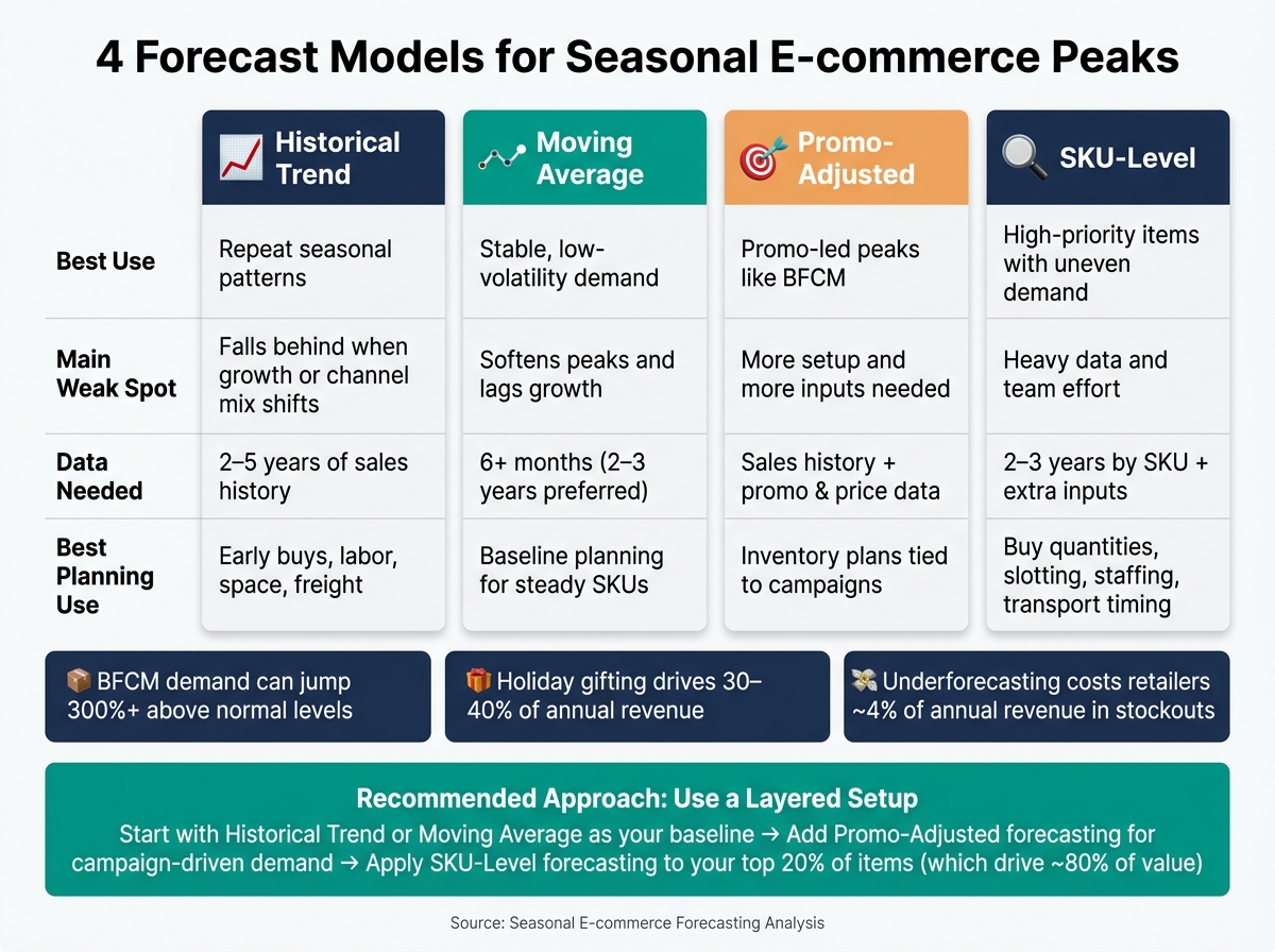
4 Forecast Models for Seasonal E-commerce Peaks: Quick Comparison Guide
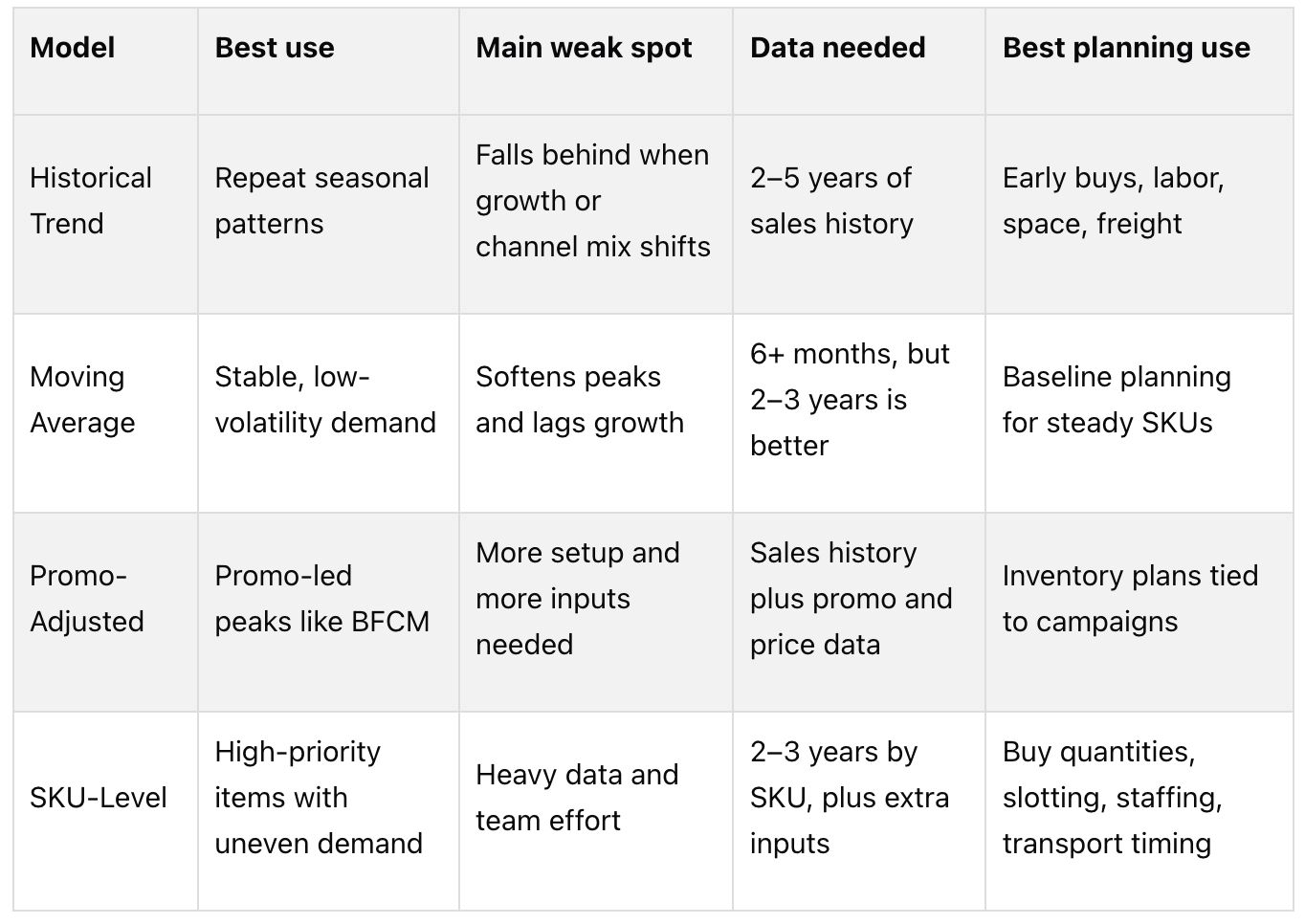 If you want the plain answer, it’s this: use a layered setup, not a single model. Start with a baseline, add promo lift where demand is campaign-driven, and go SKU by SKU for the items that matter most. That gives you a forecast you can actually use for inventory, warehouse space, labor, and carrier planning.
1. Historical Trend Forecasting
Historical trend forecasting breaks past sales into three parts: baseline, trend, and seasonality. The idea is simple. Seasonal demand tends to repeat at the category level, so past patterns can give you a solid baseline for future peaks.
Seasonal Fit
For the peak periods mentioned above, this is the easiest place to start. It works best when demand follows the calendar in a steady way.
A practical setup is to compare the same weeks across the past three years and use that pattern to build a seasonal multiplier. When you pair that with ops planning, historical models can produce high forecast accuracy during peak periods.
Growth Responsiveness
This approach fits steady, established demand. It starts to slip when growth, new SKUs, or new sales channels change the shape of the curve.
If you don’t adjust for trend, the model tends to under-forecast growing items and over-forecast declining ones. That’s the catch. And it’s why fast-growing brands often shift to models that react more quickly.
Data Requirements
To get results you can trust, you need at least two to three full cycles of clean, granular sales data. In practice, three to five years of SKU-level or product-family data is better for calculating year-over-year seasonal indices.
New products and channel shifts make this harder, since there isn’t much usable history to work with.
Planning Value
For established products, this forecast can help with planning months in advance, including:
- Procurement
- Labor
- Warehouse space
- Freight
Use this model when seasonality is steady and SKU history is clean. If growth or promotions start warping the pattern, it makes sense to shift to more granular methods. And when demand moves faster than history can show, moving-average models can give you a faster read.
2. Moving Average Forecasting
Unlike trend-based models, moving averages work best for steady demand, not seasonal spikes.
Moving average forecasting takes the average of the last few periods and uses it to estimate the next one. That helps smooth short-term noise and makes the underlying demand pattern easier to see.
Seasonal Fit
This model is a better match for flat demand. It suits mature, stable products that sell at a fairly even pace over time.
When demand jumps hard during a season, a simple moving average usually under-forecasts the peak because it mixes high-demand periods with slower periods right before them. In plain English: it softens the spike instead of predicting it. That’s why moving averages are better as baseline tools than as tools for peak forecasting.
Growth Responsiveness
For fast-growing brands, this model has an obvious downside: it lags behind current sales. So it often under-forecasts growing SKUs.
A weighted moving average can react a bit faster, but it still struggles with sustained growth.
Data Requirements
A 6-month moving average needs at least 6 months of data. But a longer history - usually 2 to 3 full years - gives you a better read on what’s a real pattern and what’s just noise.
It also helps to flag promotional spikes in the data. If you don’t, the model treats those spikes as part of the average, which can skew the baseline after the promotion ends.
Planning Value
Moving averages are most useful as a baseline prediction tool for stable, non-volatile SKUs that don’t swing hard because of promotions or seasonality.
Because the model can’t account for surprise spikes on its own, teams often pair it with safety stock calculations. Use forecast error to set safety stock.
When promotions are driving the spike, move to promo-adjusted forecasting.
3. Promo-Adjusted Forecasting
Moving averages can flatten a Black Friday spike. Promo-adjusted forecasting handles that problem by splitting baseline demand from promotional lift. Instead of smoothing everything into one line, it treats normal demand and promo-driven demand as two separate parts.
Baseline demand is the repeatable, calendar-based pattern. Promotional lift is the extra demand caused by discounts, email sends, paid ads, or marketplace deals. This model forecasts each one on its own.
Seasonal Fit
This approach works well for seasonal peaks because it separates calendar demand from promotion-driven lift. In practice, planners often use year-over-year seasonal indices from the last 3–5 seasons to set a steady baseline. Then they layer in lift percentages for each promo channel and record those as planning assumptions.
That split matters. If you treat a one-off promo spike like normal demand, next year’s baseline can get pushed too high even when no promo is on the calendar.
Growth Responsiveness
For fast-growing brands, the big draw is speed. AI-driven versions use demand sensing, or real-time purchase signals, to update the forecast while a campaign is live instead of only before launch. Companies using AI-based demand forecasting report a 15–25% improvement in forecast accuracy and 30% faster replenishment cycles.
Data Requirements
This model needs more than just past sales. It also relies on promo calendars, price changes, and outside signals like competitor promotions, market intelligence, and social sentiment.
At a minimum, you need 2–3 full seasons of data to separate a real seasonal trend from a one-time promo spike with some confidence. Without that history, the model can misread a short burst in demand as a pattern that will happen again. The main risk is simple: treating an old promotion like baseline demand.
Planning Value
The upside is practical: lower excess inventory and better cash flow. Businesses that use advanced forecasting methods see a 20–30% drop in excess inventory. When inventory plans line up with the marketing calendar, teams deal with fewer emergency purchase orders and get steadier cash flow.
This matters most for top-volume SKUs, the roughly 20% of SKUs that drive around 70% of sales. For those products, the added complexity is usually worth it.
When peak demand shifts hard from one product to another, the next move is SKU-level forecasting.
4. SKU-Level Forecasting
When peak demand doesn’t hit every product the same way, forecasting has to go deeper. At that point, promotion-level lift isn’t enough. You need item-level variation.
SKU-level forecasting looks at each item on its own and breaks its sales history into peak, shoulder, and off-season windows. That matters because products rarely move in lockstep. One SKU may spike hard during a seasonal rush, while another stays steady or tapers off.
Seasonal Fit
The big win here is simple: risk changes by SKU and by season, so safety stock should change too.
Demand variability shifts across the year and across items. If you use one annual standard deviation for everything, you flatten those swings into a single average. That hides peak-season risk and off-season excess.
By calculating a period-specific standard deviation (σ_period) for each part of the season, planners can set safety stock that fits the risk level of that specific window. For peak-season buy planning, that makes a big difference. Peak season safety stock for some SKUs can run as much as 8 times higher than off-season levels. A single annual average lands in the middle and misses both ends.
Growth Responsiveness
For fast-growing brands, SKU-level models pick up short-term changes that category-level forecasts gloss over.
When growth is uneven across a catalog, category-level views blur what’s happening underneath. Some items are taking off. Others are leveling out. Item-level forecasting brings those shifts into view early enough to do something with them, instead of spotting the change after inventory is already out of sync.
Data Requirements
SKU-level forecasting usually needs at least 2–3 years of item-specific sales history to separate seasonal movement from actual year-over-year trend. Without that history, it’s hard to tell whether a jump came from seasonality or from a lasting shift in demand.
For new SKUs, teams often rely on proxy data from similar items or category benchmarks. The forecast also gets sharper when you layer in:
- promotional calendars
- lead time history
- real-time external signals like weather data and Google Trends
These inputs help fine-tune the picture, especially when demand moves for reasons that don’t show up in sales history alone.
Planning Value
SKU-level forecasting matters most for A-items, where forecast accuracy directly affects buy quantities, slotting, labor, and freight timing.
And the impact doesn’t stop at purchasing. More accurate SKU-level forecasts also shape warehouse slotting, fulfillment labor planning, and transportation capacity. That includes inventory phasing, like booking sea freight months ahead and holding air express for flexible reserve inventory.
That kind of item-level detail is a big reason SKU forecasting often outperforms broader models during seasonal peaks.
Strengths and Tradeoffs by Model
At this point, the issue isn’t defining each model. It’s seeing what each one gives up.
Every model is built to handle a certain kind of planning problem. But none can cover every peak-season need. So the best fit comes down to what matters most in the moment: simplicity, speed, or SKU-level precision.
Historical trend forecasting works best when peak patterns repeat cleanly from one year to the next. That makes it useful for early buying, labor planning, and freight planning. The downside is lag. It can’t react when demand breaks away from the old pattern, which can push teams into reactive moves like expedited freight.
Moving average forecasting is good at smoothing out noise, but there’s a catch: it also softens seasonal spikes. It assumes demand stays fairly steady, and that assumption falls apart during peak season. The forecast ends up trailing the spike, and warehouse teams are left scrambling. On top of that, one annual variance number can mask two very different problems: peak-season risk and off-season excess.
Promo-adjusted forecasting deals with that problem by bringing in external signals before demand shifts. It tends to handle promo-led demand better because it separates baseline demand from incremental lift. That timing matters when inventory and media spend need to move in sync. It can also help lean 3PL operations run with less extra buffer stock. The tradeoff is complexity. To work well, it needs connected systems and demand-sensing capability.
SKU-level forecasting gives you the most precision, but it also asks the most from your data and your team. Its main edge is item-level accuracy. That matters most for high-volume A-items, where forecast error has a direct effect on inventory and service risk. For those products, better accuracy shapes buy quantities, regional inventory placement, and reorder points. The next step is to match each model to the peak scenario where it fits best.
Which Forecast Model Fits Seasonal E-commerce Peaks Best?
The right model depends on three things: demand stability, promo intensity, and SKU complexity.
If your demand pattern is steady from year to year, historical trend is often a good fit for seasonality. Moving average helps smooth out baseline noise. Promo-adjusted forecasting works better when campaigns, discounts, or product launches push demand up. And SKU-level forecasting turns broad projections into item-level inventory and fulfillment plans, which matters most for the 20% of items that often drive 80% of total value.
When demand shifts fast, last year’s sales stop being a clean guide for what’s coming next. In that case, brands need more than a backward look. Blending historical data, market trends, and AI can help line up inventory with demand and cut the odds of overstocking or stockouts.
A simple way to handle it:
- Use historical trend or moving average as your baseline
- Add promo adjustments when campaigns or launches are likely to change demand
- Apply SKU-level forecasting to your highest-value items
This layered setup helps lower the risk that comes with weak inventory control, which costs e-commerce sellers about $1.1 trillion per year. A flexible 3PL network can then turn that forecast into inventory, labor, space, and transportation plans when peak season demand moves faster than any single model can track.
FAQs
Which forecast model should I start with?
Start with the historical data method. Looking at past sales helps you spot trends and seasonal patterns, which gives you a solid baseline for planning and a first estimate of high- and low-demand periods.
As your e-commerce brand grows, you can build on that baseline with AI-powered tools or hybrid models that account for variables like promotions, social sentiment, and weather.
How do I forecast for fast-growing SKUs?
For fast-growing SKUs, older forecasting methods often miss the mark. The main reason is simple: there isn’t much sales history to work with. In these cases, AI-driven forecasting can help by grouping similar products and using those patterns to make earlier predictions with more confidence.
It also helps to mix sales data with real-time signals, such as social media sentiment, promo calendars, and market trends. Hybrid models that combine statistical methods with machine learning tend to do a better job with demand that swings hard or doesn’t follow a neat pattern.
When is SKU-level forecasting worth it?
SKU-level forecasting starts to make sense when inventory is too complex for spreadsheet-based planning. That usually happens when you're managing thousands of items across multiple channels or warehouses. At that point, a spreadsheet can only take you so far.
Done well, it helps you spot which products are heading toward stockouts and which ones are drifting into overstocking. It can also improve slotting and picking efficiency, which matters a lot when warehouse teams are moving fast and small delays add up.
This kind of forecasting is also useful for fast-growing brands or volatile products. Instead of leaning only on past sales, you can use external signals and real-time data to react faster when demand shifts.
Related Blog Posts
Related Articles
7 WooCommerce 3PL KPIs Teams Track

Centralized vs Decentralized Replenishment
